
We’ve had several requests to add more technical posts to the blog, so we’re kicking off with a Technical SEO series designed to help you make the most of your time. Search engine optimisation has become more data-driven than ever thanks to tools like Google's Webmaster Tools, Majestic SEO, Open Site Explorer and many others.
This means that SEOs are now dealing with organising, analysing and trying to get meaningful information from mountains of data. It’s hard work. However, it can be made much easier with Excel which is an absolute godsend to SEOs when used to its full potential. Why? Because with Excel almost everything can be automated, which means you’ll save so much time on repetitive SEO tasks.
So, if functions like VLOOKUP, CONCATENATE and IFERROR make you scratch your head, read on to learn how to use Excel to supercharge your SEO on a daily basis.
It’s these Excel functions that we’ll be covering in Part 1 of Excel for SEO and learning how to use them will make your keyword research task so much easier and time effective.
Let’s get started…
Preparing the data
After you’ve done your keyword research and exported your list of keyword ideas into an Excel spreadsheet, you’ll need to clean it up so you won’t have to work with more values than necessary.
The following are easy steps for sorting out your data and getting a bit more organised.
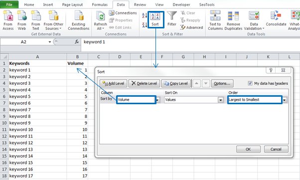
For example, you could sort your tables based on search volumes, from highest to lowest. To do that, click on Sort -> Sort by Volume -> Order Largest to Smallest.
We recommend removing duplicates from combined sets of data. Click on Remove Duplicates and then choose which column you want to remove the duplicates from, in this case Keywords.

Next, you should use filters to sort your data and organise it into smaller sets of data. To do that, select your table and click the Filter button:

You will see different options that allow you to sort your data, including alphabetically, by colour, by text. In this example, we will filter the results by keywords that include the word “red”.
Click on Text Filters -> Contains:


Add the word you want all the results to include, in this case red, and click OK.
Now all the keywords displayed in the table will include the word “red”:

This is helpful for separating lists of keywords by products, services or other characteristics.
Creating lists of keywords
The following special operators will enable you to speed things up when building your lists of keywords and keyword phrases.
For this task you will need to know how to use:
& – Concatenation symbol – This operator allows you to combine two cells into one. You can add the & sign between strings of text in quote marks or between cell numbers.
Watch the video to see an example:
$ – Use this symbol if you want a formula's column and/or row value to stay the same when you drag the formula into other cells.
Watch our video to see how to use the $ sign in Excel:
Ok, now that you know how these two basic symbols work, let’s look at how you can use them to build your keywords list:
Comparing data from two different tables
Next we're going to look at using the VLOOKUP command to compare data from two separate tables. In this case, VLOOKUP searches the first column of a table for a certain value and if a match is found it returns the value contained in a specified column in the same row as the match.
Here's the information you need for the VLOOKUP formula, followed by a closer look at each element of the command:
VLOOKUP (lookup_value, table_array, col_index_num, [range_lookup])
Lookup_value – The value you want to search for. This might be a word or a number depending on the kind of data you're looking at.
Table_array – This tells the formula the location of the table you want to look at.
Col_index_num – This is the table column which will return data when your lookup_value is found.
Range_lookup – This tells Excel to do an exact match or a partial match when searching. True returns partial matches and false exact matches.
Let's look at a simple example. Here we have a basic table with keywords in column one and rankings in column two. Now we want a formula that will return the ranking for a specific keyword – let's say “keyword4”.
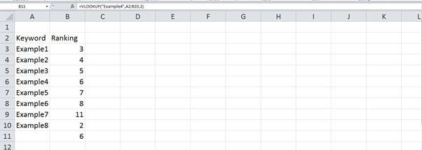
You can see the formula, VLOOKUP(“Example4”,A2:B10,2), returns the value of “6” in cell B11, which is correct. VLOOKUP is not extremely useful for small tables like this. However, if you're dealing with large tables, then VLOOKUP is invaluable.
But what if you have more than one table? Let's see how you can use VLOOKUP to work with several sets of data.
In this example, we have two tables – one of our rankings and one of a competitor's rankings. We can use VLOOKUP to quickly combine the two sets of data.

As you can see, the formula in C3 is more complex than in our first example, but the principle remains the same. This time we have VLOOKUP(A3,$E$3:$F$10,2,FALSE).
Let's consider the differences:
- The lookup_value – In our first example, we looked at a specific keyword. In the second example, we're referring the formula to cell A2.
- The table_array – In this example, we're using our competitor data as the table_array. We have also added “$” in front of the column and row references.
- Range_lookup – We have set this to FALSE to ensure only the exact keyword is matched.
- We have dragged the formula down from cell C3. This means we have a formula that searches the competitor data for all of our keywords and returns their ranking. (NB if we had not set the lookup_value to A2 or used “$” for the table_aray field, then dragging the formula would not have worked).
However, there is still something wrong. Our competitors don't rank for exactly the same keywords as us. In this case, there's no match for the keywords “Example4, Example5 and Example6”. That's why the “#N/A” value shows up in three cells.
To fix this we can use the IFERROR function. As the name suggests, this allows you to display a specified value if a formula returns an error.
Here's what it looks like: IFERROR (value,value_if_error)
“Value” is the formula you want to check for errors (in this case the VLOOKUP formula we've just put together) and “value_if_error” is what you want the output to be if there is an error. Let's say that's “No data”.
Put that all together and the formula we get is IFERROR(VLOOKUP(A3,$E$3:$F$10,2,FALSE),”No Data”)
Pop that in cell C3, drag it down and here’s what you’ll get:

Things you should know:
- The tables don’t have to be in the same sheet and they can be in separate tabs.
- The keyword you’re searching for should be found in the first column of the second table. The VLOOKUP formula can only match values with the first column.
- Always add $ to lock certain values and keep them in place.
Have you used any of these operators and formulas before? If not, let us know how you get on with our guide in the comments!